Tab Processing
The processing tab is the most complex tab of goGPS And for this reason, it requires is one description page. Here the user can manipulate everything from the data selection to the filtering of the observations to the definition of the full parametrization of the least-squares adjustment.
This tab is divided into 6 tabs
- Tab Data Selection
- Tab Atmosphere
- Tab Pre-Processing
- Tab Generic-Options
- Tab PPP Parameters
- Tab Network parameters
To see other tabs go back to the index of the Settings
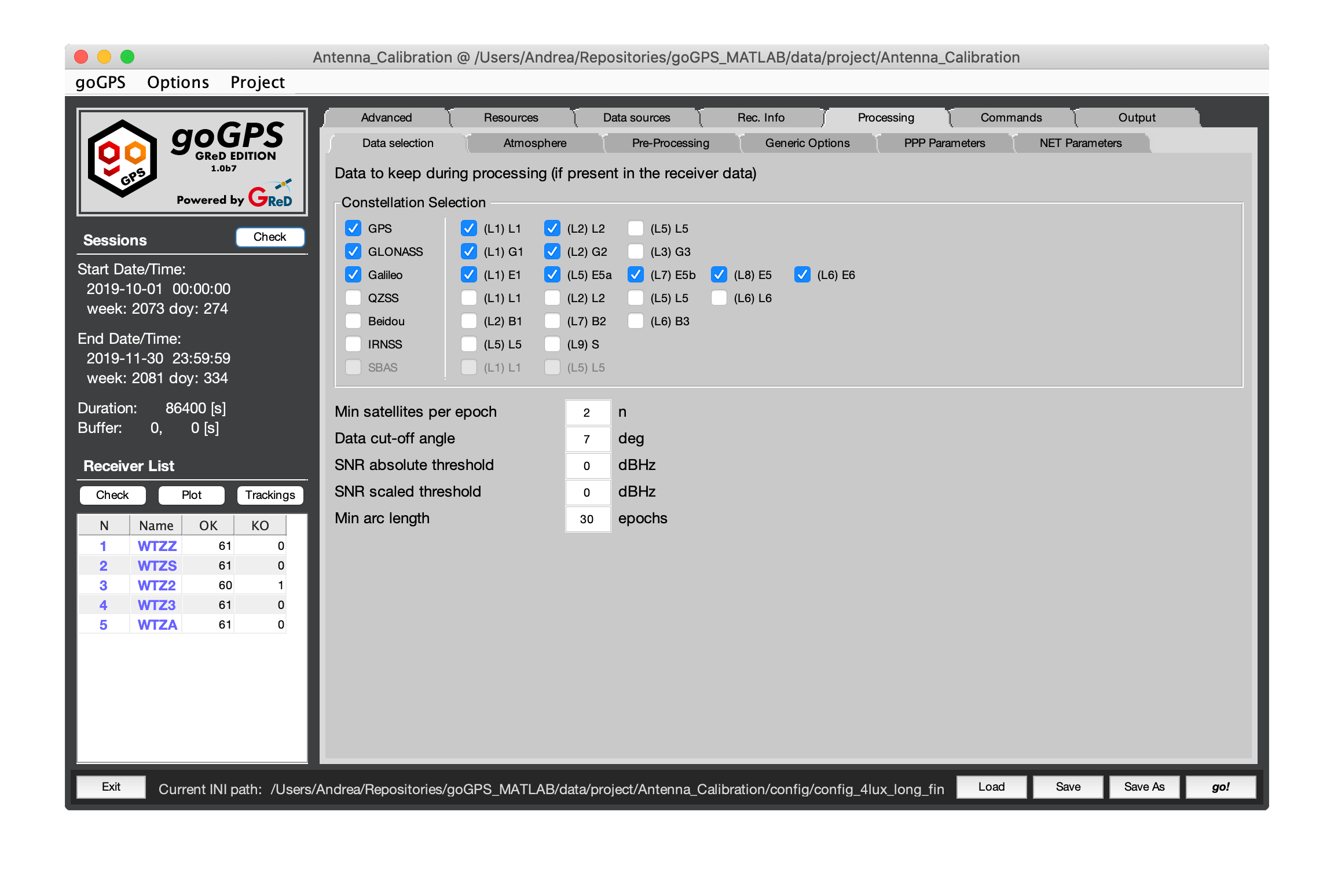
Tab Data selection
In this tab, the user can set the options for the data selection.
Constellation Selection
this panel allows to activate and de-activate some satellite systems/frequencies.
Note:
- the user needs to select the proper orbits for the enabled constellations (e.g. use MGEX orbits when various systems are selected);
- when processing with the combined engine only the best frequencies are used for creating an iono-free combination;
- be aware that due to the inter-frequency clock bias with L5 not automatically handled by goGPS, selecting GPS L5 may produce bad results;
- to use more than two frequency at a time the uncombined engine must be used for the processing;
- if a frequency/constellation is not present in a receiver goGPS should be able with the remaining observables.
Data exclusion
- "Min satellite per epoch" - under this threshold the epoch is discarded from the processing (default value is 2).
- "Data cut-off angle" - during the preprocessing, after the estimation of a good position of the receiver, all the observations of a satellite below this elevation are deleted from the workspace and not considered in the rest of the processing.
- "SNR absolute threshold" - Signal to Noise Ratio provides a good insight on the quality of the observations registered by the receiver, in particular, it is severely affected by multipath. When this index goes below a certain value it indicates that the observations (especially the pseudo-ranges) might be degraded, setting a threshold allows goGPS to discard these bad data. For more information see the function remUnderSnrThr in Receiver_Work_Space.m.
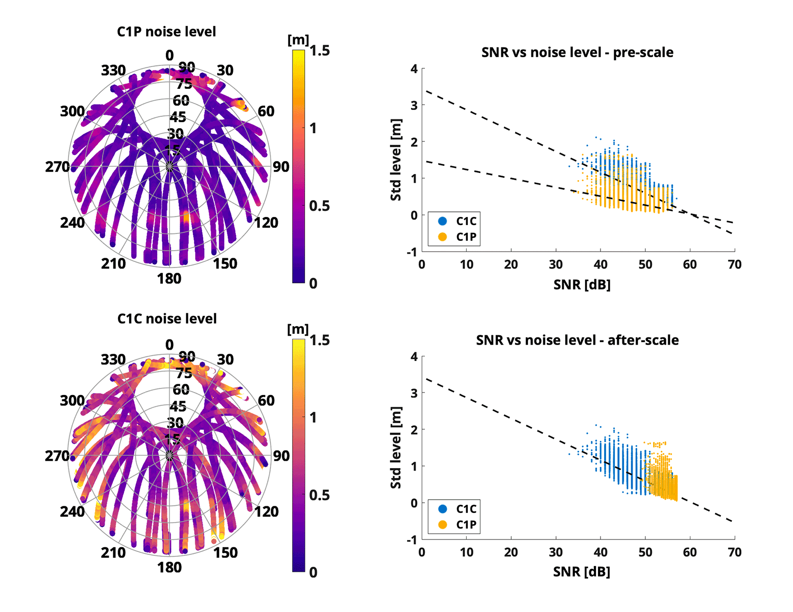
- "SNR scaled threshold" - different trackings (e.g. GPS C1C, C1W or GLONASS C1P and C1C) and different frequencies have different SNR scaling. Setting a threshold on 28dB might be good for one tracking, but the same value for another could delete too many values. goGPS try to rescale all the SNR from different systems/frequencies/trackings to the one of C1C (or comparable) to be able to set up a unique SNR limit valid for all the observables instead of setting a different one for each observable. A value between 25-32 dB is generally good. To scale the SNR a rough estimation of the pseudo-ranges noise is performed reducing the data with their synthetic version, biases are removed and the standard deviation of the residuals is computed on a moving window arc by arc. Pseudo-ranges below the threshold are deleted from the receiver before the last estimation of the code-only solution in pre-processing. For more information see the function remUnderSnrThr in Receiver_Work_Space.m. In the following figure, the level of noise of a WTZZ (Wetzel) station for GLONASS C1 is compared, C1P has lower noise but also lower SNR, its SNR is scaled to have similar values for the same level of noise of C1C.
- "Min arc length" - goGPS will delete any arc smaller than this value, the number is expressed in epochs and not seconds. Remember that the ambiguity of a small arc is generally badly estimated, a reasonable value for this parameter in a 30 seconds processing is 10-12 epochs.
Go back to the Index of contents
Tab Atmosphere
This tab is used to select the options for better management of the atmospheric effects. This information is needed wether or not the troposphere will be estimated.
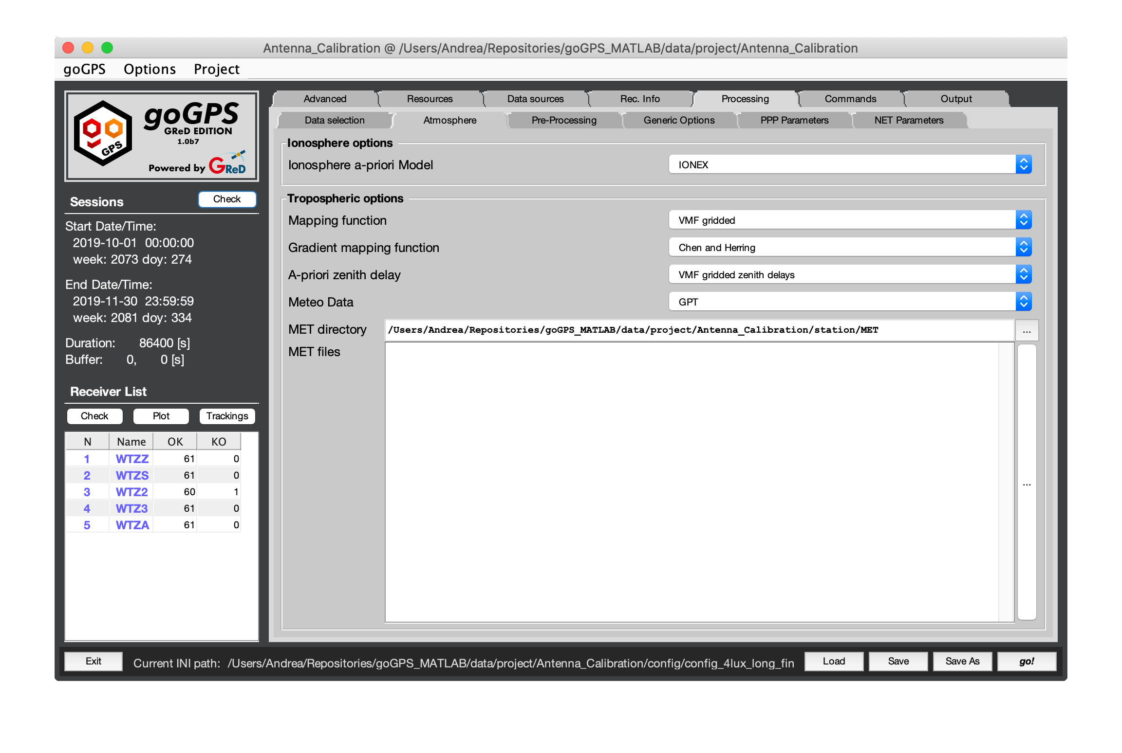
Ionosphere options
- Ionosphere a-priori Model - in this pop-up menu the user can select the type of a-priori model to be removed from the observations. A good model helps the outlier-detection and pre-processing phase. The available options are:
- 1 - none
- 2 - Klobuchar - standard Klobuchar model, it requires ionospheric parameters that are usually read from broadcast orbits (goGPS can automatically fetch them)
- 3 - IONEX - this is the most precise model that can be applied, it is read from IONEX files, depending on the preferred type selected in the resources tab it can be a model from observed values or just a prediction.
Tropospheric options
- Mapping function - in this pop-up menu it is possible to select the tropospheric mapping function, at the moment only 3 models are available, the additional model can be implemented into Receiver_Work_Space.getSlantMF.
- 1 GMF - Global Mapping Function
- 2 VMF gridded - Vienna Mapping Function (they are automatically downloaded when needed)
- 3 Neil - Niel Mapping Function
- Mapping function gradients - in addition to the tropospheric mapping function for estimating zenith delays, it is possible to specify the mapping function for the gradients.
- 1 Chen and Herring
- 2 MacMillan
- A-priori zenith delay - this is the a-priori model to be used for computing tropospheric delays, two options are available:
- 1 Saastamoinen from meteo data - this option makes goGPS use as a-priori model Saastamoinen, the origin of the data to be used depends on the next field in the GUI
- 2 VMF gridded zenith delays - these are Zenith delays coming from the Vienna gridded maps of ZTD
- Meteo Data - here the user can select the source of the meteorological data to be used:
- 1 Standard Atmosphere - Standard values of Pressure (1013.25 mbar), Temperature (18 °Celsius), Humidity (50 %)
- 2 GPT - Global Pressure Temperature
- 3 MET files - use the Meteorological RINEX specified in the following fields.
- MET files - goGPS can use meteorological RINEX files to import temperature, pressure, and humidity from meteorological stations. It automatically interpolates the data at the right elevation and station positions (See Meteo_Data.getVMS for more details). The syntax for these files are like
Go back to the Index of contents
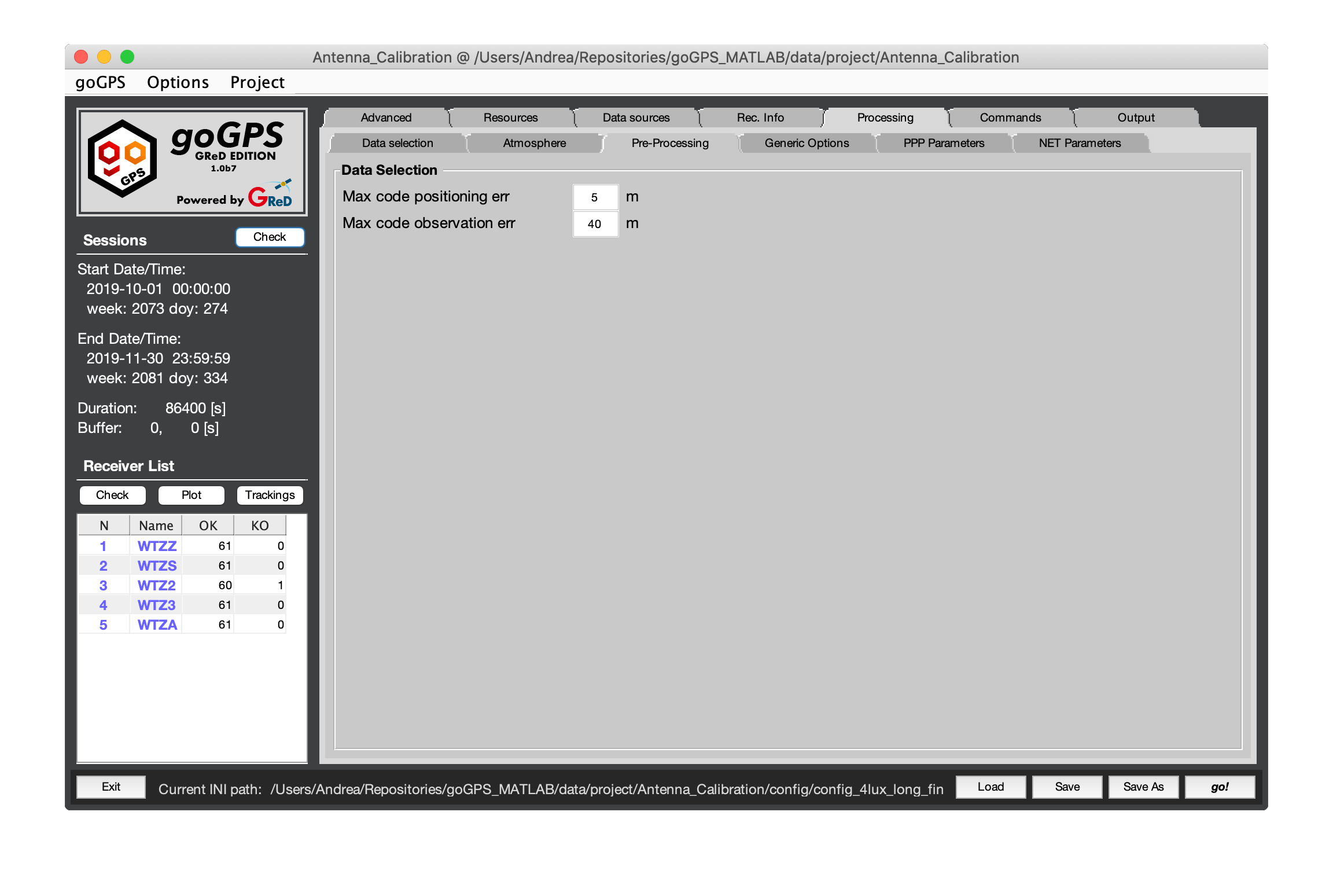
Tab Pre-processing
In this tab, the user can select options that modify how the pre-processing works.
-
"Max code positioning error" - if the pre-processing of a station returns a sigma0 (from the LS adjustment) larger than this value, the station is considered having problems, pre-processing fails and PPP or network adjustment can not be computed.
-
"Max code observation error" - all the pseudo-range observations having a residual from the last step of pre-processing larger than this value are deleted and a new LS adjustment is performed without them.
Go back to the Index of contents
Tab Generic Options
This tab contains all the parameters that might influence PPP or Network processing but are not related to the parametrization of the least-square adjustment.
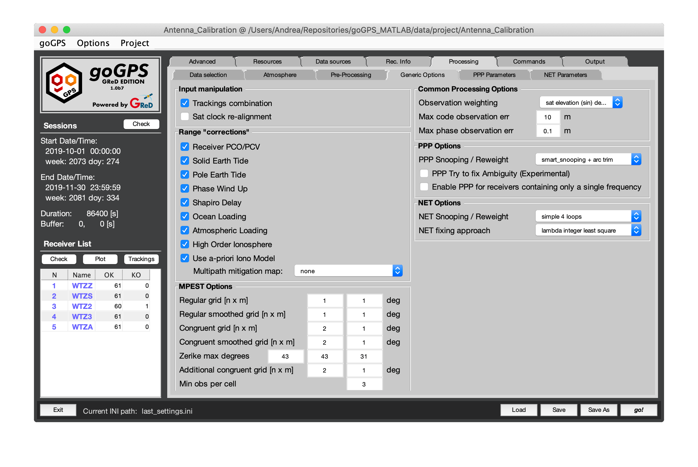
Input manipulation
In this section, the receivers observations and the satellite clocks can be modified
-
"Trackings combination" - when this flag is selected carrier-phase observations from multiple trackings of the same frequency are combined using their approximate noise levels as weights, tracking biases and cycle-slips not present on all the trackings are estimated and corrected (experimental - default "on"). For more details see the function combinePhTrackings in Receiver_Work_Space.m. To estimate the noise level of each carrier-phase (ph) and then the weights the following algorithm is applied:
using the position computed at the end of pre-processing (code positioning) compute the synthesized pseudo-ranges (_spr_) for the satellites seen by the receivercompute the residuals: _ph_ - _spr_remove relative tracking biasescompute the moving variance (5 epoch window) for each tracking of the same observable (e.g. L1C L1W)compute a cubic interpolation of the variance with respect to the elevationcompute the weight as 1 / this interpolated index
-
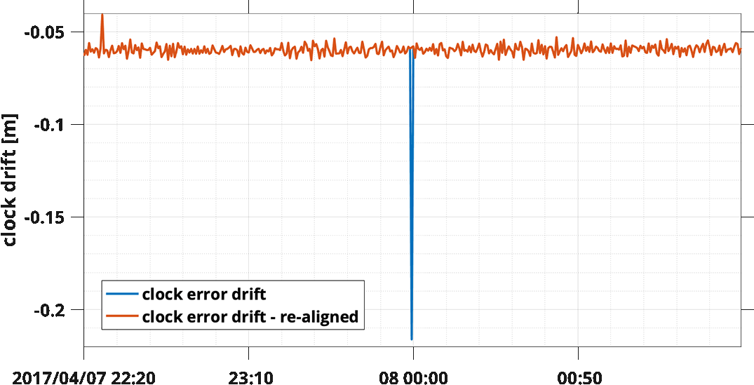
"Clock re-alignment" - the satellite clocks estimated by many providers have severe jumps at the end of the day. These are spanning from some centimeters to a few meters; selecting this flag goGPS will try to compensate and correct this jumps (experimental - default "off"). This effect is probably due to the independent estimation of the clock errors among different days. For more details see the function addClk in Core_Sky.m. Here follows an example of this jump, seen as a spike in the clock drift of a satellite (expressed in meters):
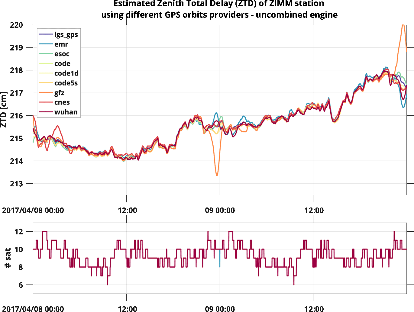
The effect of this flag influences the solution near midnight GMT when two sets of old and new ephemeris connect. Removing this jump improves the smoothness of the orbits and thus the outlier detection phase that otherwise may find false-positive outliers. In the following example using different orbit providers and processing the ZIMM (Zimmerwald) station with the PPP uncombined goGPS engine we can see how the orbit of GFZ and CNES produce larger deviation in the estimated ZTD with respect to the other solutions:
when the re-alignment flag is selected the solutions change showing the following behaviors:
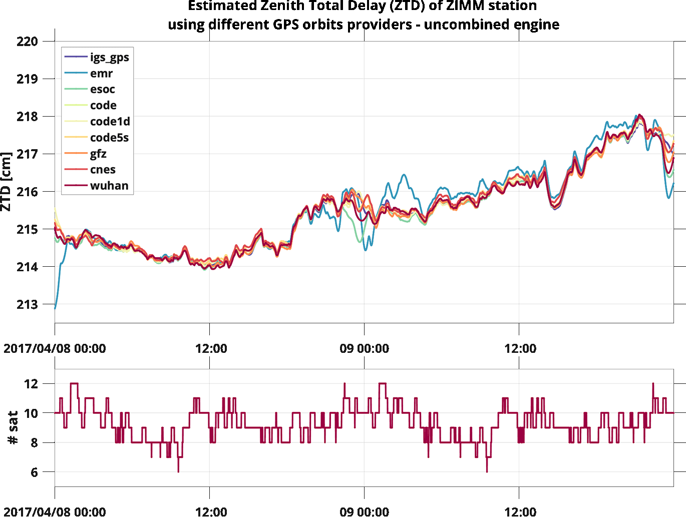
solutions computed with GFZ and CNES orbits improve, while some of the others are now worse. Use this flag carefully checking case-by-case if this adjustment improves the solution.
The correction algorithm at the moment is very simple and works as follows:
Take 200 epochs at the left of the file change epoch, and 200 at the rightcompute std of the drift of the two subsets of dataif the jump is greater than the standard deviation compute a correction(correction) perform a linear interpolation of the two subsets predicting one epoch of the clock from the two sides and offset the right side to minimize the jumpAn offset in a satellite clock in a network solution causes no problems, while in PPP might influence the ambiguity estimation of an arc, this correction is still experimental and needs additional investigations to be applied safely.
Range corrections
This panel allows applying all the corrections needed for a Precise Positioning. All the corrections are applied at the end of the pre-processing phase. Although all these corrections are not necessary for a network adjustment, applying them allows a better outlier detection. Among all the available corrections "Atmospheric Loading" and "High Order Ionosphere" are the ones with a lesser impact and can be disabled safely. The list of corrections that can be applied to the GNSS observations are:
- "Receiver PCO/PCV" - phase center offsets and variations, the magnitude of this effect depends on the antenna type
- "Solid Earth Tide" - tides due to Earth's crust movements (tens of centimeter).
- "Pole Earth Tide" - tides due to the wobbling of the Earth rotation axis (up to 2.5 cm vertical - 0.7 cm horizontal).
- "Phase Wind Up" - affect only phases due to the electromagnetic nature of circularly polarised waves, it depends on the relative orientation of satellite and receiver antennas (some centimeters).
- "Shapiro Delay" - relativistic effect (less than 2 cm).
- "Ocean Loading" - due to ocean tides deformations of the seafloor and a surface displacement of adjacent land (few centimeters).
- "Atmospheric Loading" - this effect is due to the variation of the atmospheric pressure.
- "High Order Ionosphere" - effect due to the second, and third-order due to the signal passing through the ionosphere.
- "Use a-priori Iono Model" - effect of ionosphere computed with the model selected in the Athmosphere tab, this is very useful in case of ionospheric interpolation.
- "Multipath mitigation" - with this pop-up menu the user can choose to try to mitigate multipath using previously generated multipath maps. It is possible to choose between a map based on a Zernike polynomials expansion (smoother) or the version with restored the higher frequencies of staking the residuals, see the command section Multipath management for further details.
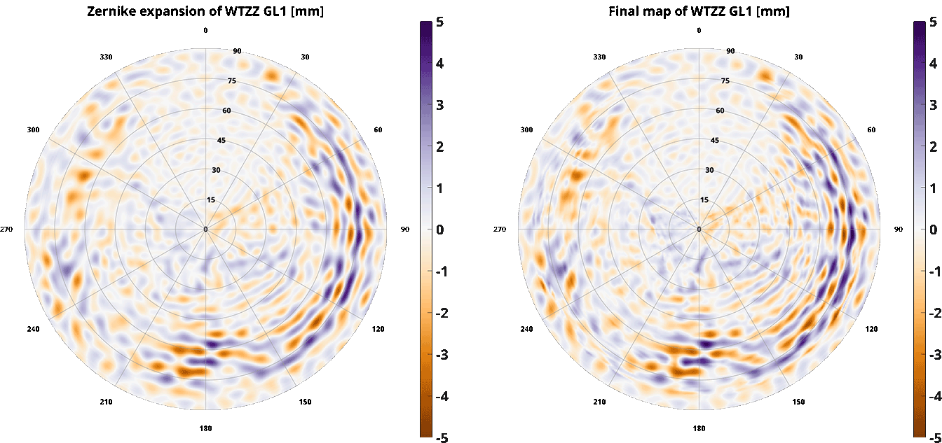 On the left the smoother solution, on the right the highest details of the staking are preserved
Go back to the Index of contents
MPEST Options
This section is dedicated to the settings for the creation of the multipath maps, for more information see also: Multipath management. 6 grids are created by goGPS each with his own positive and negative aspects. Here follows the main settings for their creation, set them to zero to avoid their calculations:
- Regular grid [n x m] dimension of grid in degrees. This is the simplest gridding with costant dimension cells in azimuth and elevation.
- Regular smoothed [n x m] dimension of this grid in degrees. With respect to the first grid this uses additional pseudo observations in empty cells and the final result is upscaled to a 0.5 x 0.5 degree grid.
- Congruent grid [n x m] set the dimension of this grid in degrees. This is a congruent cells grid, meaning that increasing the elevation the number of cells decreases (they get larger in azimuth). This grid is then scaled to a regular grid.
- Congruent smoothed grid [n x m] set the dimension of this grid in degrees. Similarly to the regular smoothed this grid is upscaled to a regular 0.5 x 0.5 degree grid
- Zernike max degrees set the degree of expansion to create a 0.5 x 0.5 smooth regular grid. The three entries are three expansions that can enhance the frequency close to the horizon, to the middle elevations and to the zenith.
- Additional congruent smoothed grid [n x m] set the dimension of this grid in degrees. This grid is upscaled to a regular 0.5 x 0.5 degree and summed to the Zernike grid.
- Min obs per cell For non Zernike gridding this represent the minimum number of observations per cell to get a valid value. If this threshold is not reached the cell will be set to zero.
Go back to the Index of contents
Common Processing Options
- "Observation weighting" - Select the type of observation weighting function. These are the available options:
- uniform - all observations equally weighted
- satellite elevation $sin(el)$
- square of satellite elevation $sinn(el)^2$
- "Max code observation err" - the pseudo-range observations having residuals above this threshold are excluded from the LS adjustment (this threshold works only for the uncombined engine).
- "Max code observation err" - the carrier phase observations having residuals above this threshold are excluded from the LS adjustment.
PPP Options
These options are dedicated to the Precise Point Positioning adjustment.
- "PPP Snooping / Reweight" - This pop-up menu allow the user to chose different types of outlier rejection / data re-wight. The list of methods currently available is:
- 1 - none perform neither snooping nor reweight
- 2 - re-weight Huber see Table2 in Gökalp et al, 2008 - Evaluation of Different Outlier Detection Methods for GPS Networks is applied on all the observations having residuals greater than a threshold level, set to be 2 * std(residuals)
- 3 - re-weight Huber (no threshold) Huber M-estimator applied on all the residuals
- 4 - re-weight Danish see Table2 in Gökalp et al, 2008 - Evaluation of Different Outlier Detection Methods for GPS Networks is applied on all the observations having residuals greater than a threshold level, set to be 2 * std(residuals)
- 5 - re-weight DanishWM Modified Danish M-estimator, is applied on all the observations having residuals greater than a threshold level, set to be 2 * std(residuals)
- 6 - re-weight Tukey see Table2 in Gökalp et al, 2008 - Evaluation of Different Outlier Detection Methods for GPS Networks is applied on all the observations having residuals greater than a threshold level, set to be 2 * std(residuals)
- 7 - simple snooping all the observations having residuals greater than 2.5 * std(residuals) are removed from the adjustment
- 8 - smart snooping it's a method based on two threshold levels, the first one triggers the removal of the observations until its residuals re-enter below the second threshold (e.g. detection on 6 sigma0, removal of data till their residuals are below 2.5 sigma0).
- 9 - smart snooping + arc trim like the previous but the second threshold is lower (2 * std(residuals)), furthermore, all the arc edges having residuals greater than 2 * std(residuals) are removed
- "PPP Try to fix Ambiguity (Experimental)" - when this flag is enabled the PPP engine will try to fix ambiguities, note that this option at the moment works only with CNES orbits (they provide BIASes), receivers with precise code, and the combined engine.
- "Enable PPP for receivers containing only a single frequency" - by default goGPS does not compute any PPP solutions for single frequency receivers due to the high ionospheric errors that might be introduced. In some cases, the ionospheric delay is removed from the observations by interpolation or models and the user might want to re-enable the PPP processing.
Network Options
These options are dedicated to NETWORK adjustment.
- "NET Snooping / Reweight" - Network snooping and reweight have not been fully implemented. A different strategy is applied here: the uncombined engine just disregard all the observations set above the limit for maximum phase and code residuals in the generic options (see
Network.adjustNewfor more details); the combined approach instead have three options:- 1 - none perform neither snooping nor reweight
- 2 - simple 4 loops - this procedure removes outliers iteratively on residuals. At first, try to remove the worse data till the solution (in maximum 4 iterations) converges to a final adjustment (see
Network.adjustfor more details) - 3 - 4 loops + remove bad satellites In addition to the previous approach, goGPS remove "bad" satellites, i.e. all the observations having residuals not having zero mean (see
Network.adjustfor more details)
- "NET fixing approach" - select the fixing approach to be used (remember that to use lambda3 you need to have requested the code for applying it), the current options are:
- 1 - none
- 2 - lambda3 search and shrink
- 3 - lambda3 integer bootstrapping
- 4 - lambda partial
- 5 - bayesian
- 6 - bayesian best integer equivariant
- 7 - sequential best integer equivariant
Go back to the Index of contents
Tab PPP Parameters
In this tab, the user can set the parametrization for the PPP processing.
Note: The term regularization is used for Tykhonov regularization also known as ridge regression or as L2 regularization, it is implemented by pseudo-observation.
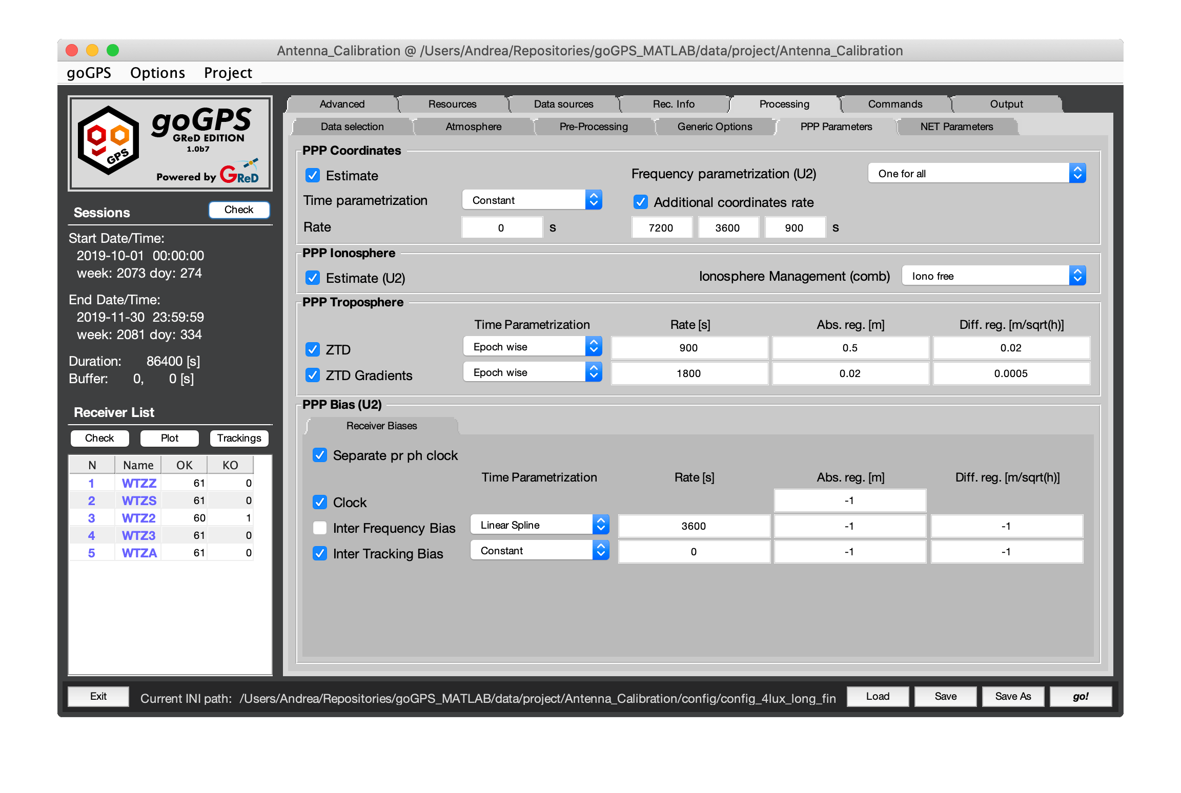
Coordinates
The parametrization of the coordinates can be set in this panel
- Estimate - This tick box will determine if the coordinates are estimated or not in the adjustment.
- Time parametrization - This pop up let the user choose the type of time parametrization wanted, the available options are:
- 1 - Costant - One set of coordinates for the whole session.
- 2 - Epoch wise - One set of coordinates per epoch.
- 4 - Regular spaced constant - Sets of coordinates spaced regulary
- 5 - Linear spline - Linear spline
- 6 - Cubic spline - Cubic spline
- Rate - Temporal rate of the parameter.Ignored if Time parametrization set to constant
- Frequency parametrization - This pop up will let you choose the possible parametrization in term of frequency and tracking (Only in uncombined mode)
- 1 - Per tracking - One set of coordinates for each different tracking.
- 2 - Per frequency - One set of coordinates for each different frequency.
- 3 - One for all - One set of coordinates for all tracking.
- 4 - Per binned frequency - One set of coordinates for each different frequency (Glonass frequency binned per band).
- 5 - Per frequency and constellation - One set of coordinates for each frequency divided also by constellation.
- 6 - Per rinex band - One set of coordinates for each RINEX 3 band.
Ionosphere
This panel deals with the parametrization of the ionosphere
-
Estimate - This tick box will determine if the ionospheric parameter is estimated or not in the adjustment.
-
Ionosphere Management - here it is possible to select the kind of management for the ionospheric delay, this option is valid only when using the combined engine
- 1 - Iono-free - when selected goGPS uses the iono-free combination to process dual-frequency data.
- 2 - Smooth GF - when selected goGPS will use the geometry-free combination pf L1 and L2 (only these two) to compute a smooth ionospheric delay that will be removed from the observations. This is similar to using an iono-free approach but with a slightly smoother final result.
- 3 - External-model - when this option is selected (or only one frequency is logged by the receiver) no combinations are used, an a-priori external model should be applied (see tab pre-processing) to have reasonable results. The model to be used is set in the Atmosphere tab.
Troposphere
In this panel on the left column, the tropospheric parametrization can be set
ZTD - This tick box will determine if the ZTD parameter is estimated or not in the adjustment.
- Time parametrization - This pop up can be used to choose the time parametrization:
- 1 - Epoch wise - One ztd paramter per epoch.
- 2 - Linear spline - Ztd parametrized as a linear spline.
- 3 - Cubic spline - Ztd parametrized as a cubic spline.
- Rate - Rate of ZTD spline
- Absolute Regularization - Absolute regularization of each ZTD paramter by means of pseudo-observation with standard deviation equal to the value of the field
- Differential Regularization - Regularize the difference of the paramter t+1 and t with an obervation with standard deviation equal to the value of the field (unit in m/sqrt(hour))
ZTD Gradients - This tick box will determine if the ZTD gradients parameter (North and East) are estimated or not in the adjustment.
- Time parametrization - This pop up can be used to choose the time parametrization:
- 1 - Epoch wise - One set of Ztd gradients paramter per epoch.
- 2 - Linear spline - Ztd gradients parametrized as a linear spline.
- 3 - Cubic spline - Ztd gradients parametrized as a cubic spline.
- Rate - Rate of Ztd gradient spline
- Absolute Regularization - Absolute regularization of each ZTD gradient paramter by means of pseudo-observation with standard deviation equal to the value of the field
- Differential Regularization - Regularize the difference of the paramter t+1 and t with an obervation with standard deviation equal to the value of the field (unit in m/sqrt(hour))
Receiver Bias
In this panel, it is possible to parametrize the various receiver bias
- Separate pr ph clock - This tick box will separate clock by phase and pseudo-range in the adjustment
The possible parameters are organized in a tab, they are:
- Clock - Clock desynchronization
- Inter Frequency Bias - Bias between different frequency tracked by the receiver
- Inter Tracking Bias - Bias between different code tracked by the receiver
The table let the user choose the parametrization with five column:
- Estimate - This tick box will determine if the parameter is estimated or not in the adjustment.
- Time parametrization - This pop up can be used to choose the time parametrization:
- 1 - Constant - One paramter per the whole session.
- 2 - Epcoh wise - One paramter per epoch
- 4 - Regular spaced constant - Sets of coordinates spaced regulary
- 5 - Linear spline - Linear spline
- 6 - Cubic spline - Cubic spline
- Rate - Rate of paramater
- Absolute Regularization - Absolute regularization of each ztd paramter by means of pseudo-observation with standard deviation equal to the value of the field
- Differential Regularization - Regularize the difference of the paramter t+1 and t with an obervation with standard deviation equal to the value of the field (unit in m/sqrt(hour))
Go back to the Index of contents
Tab Network Parameters
In this tab, the user can set the parametrization for the network processing.
Note: The term regularization is used for Tykhonov regularization also known as ridge regression or as L2 regularization, it is implemented by pseudo-observation.
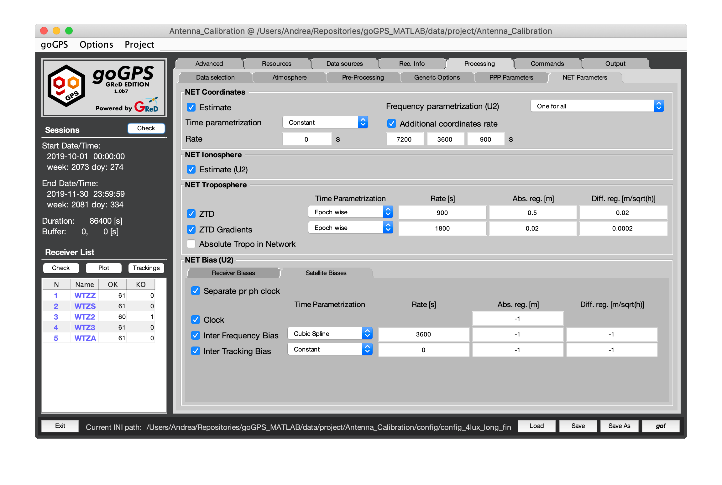
Coordinates
The parametrization of the coordinates can be set in this panel
- Estimate - This tick box will determine if the coordinates are estimated or not in the adjustment.
- Time parametrization - This pop up let the user choose the type of time parametrization wanted, the available options are:
- 1 - Costant - One set of coordinates for the whole session.
- 2 - Epoch wise - One set of coordinates per epoch.
- 4 - Regular spaced constant - Sets of coordinates spaced regulary
- 5 - Linear spline - Linear spline
- 6 - Cubic spline - Cubic spline
- Rate - Temporal rate of the parameter. Ignored if Time parametrization set to constant
- Frequency parametrization - This pop up will let you choose the possible parametrization in term of frequency and tracking (Only in uncombined mode)
- 1 - Per tracking - One set of coordinates for each different tracking.
- 2 - Per frequency - One set of coordinates for each different frequency.
- 3 - One for all - One set of coordinates for all tracking.
- 4 - Per binned frequency - One set of coordinates for each different frequency (Glonass frequency binned per band).
- 5 - Per frequency and constellation - One set of coordinates for each frequency divided also by constellation.
- 6 - Per rinex band - One set of coordinates for each RINEX 3 band.
Ionosphere
This panel deals with the parametrization of the ionosphere
-
Estimate - This tick box will determine if the ionospheric parameter is estimated or not in the adjustment.
-
Ionosphere Management - here it is possible to select the kind of management for the ionospheric delay, this option is valid only when using the combined engine
- 1 - Iono-free - when selected goGPS uses the iono-free combination to process dual-frequency data.
- 2 - Smooth GF - when selected goGPS will use the geometry-free combination pf L1 and L2 (only these two) to compute a smooth ionospheric delay that will be removed from the observations. This is similar to using an iono-free approach but with a slightly smoother final result.
- 3 - External-model - when this option is selected (or only one frequency is logged by the receiver) no combinations are used, an a-priori external model should be applied (see tab pre-processing) to have reasonable results. The model to be used is set in the Atmosphere tab.
Troposphere
In this panel on the left column, the tropospheric parametrization can be set
ZTD - This tick box will determine if the ZTD parameter is estimated or not in the adjustment.
- Time parametrization - This pop up can be used to choose the time parametrization:
- 1 - Epoch wise - One ztd paramter per epoch.
- 2 - Linear spline - Ztd parametrized as a linear spline.
- 3 - Cubic spline - Ztd parametrized as a cubic spline.
- Rate - Rate of ZTD spline
- Absolute Regularization - Absolute regularization of each ZTD paramter by means of pseudo-observation with standard deviation equal to the value of the field
- Differential Regularization - Regularize the difference of the paramter t+1 and t with an obervation with standard deviation equal to the value of the field (unit in m/sqrt(hour))
ZTD Gradients - This tick box will determine if the ZTD gradients parameter (North and East) are estimated or not in the adjustment.
- Time parametrization - This pop up can be used to choose the time parametrization:
- 1 - Epoch wise - One set of Ztd gradients paramter per epoch.
- 2 - Linear spline - Ztd gradients parametrized as a linear spline.
- 3 - Cubic spline - Ztd gradients parametrized as a cubic spline.
- Rate - Rate of Ztd gradient spline
- Absolute Regularization - Absolute regularization of each ZTD gradient paramter by means of pseudo-observation with standard deviation equal to the value of the field
- Differential Regularization - Regularize the difference of the paramter t+1 and t with an obervation with standard deviation equal to the value of the field (unit in m/sqrt(hour))
Absolute troposphere in-network - activating this flag when performing a network adjustment with long base-lines the full tropospheric delay is estimated for each station.
Receiver Bias
In this panel, it is possible to parametrize the various receiver bias
- Separate pr ph clock - This tick box will separate clock by phase and pseudo-range in the adjustment
The possible parameters are organized in a tab, they are:
- Clock - Clock desynchronization
- Inter Frequency Bias - Bias between different frequency tracked by the receiver
- Inter Tracking Bias - Bias between different code tracked by the receiver
The table let the user choose the parametrization with 5 column:
- Estimate - This tick box will determine if the parameter is estimated or not in the adjustment.
- Time parametrization - This pop up can be used to choose the time parametrization:
- 1 - Constant - One paramter per the whole session.
- 2 - Epcoh wise - One paramter per epoch
- 4 - Regular spaced constant - Sets of coordinates spaced regulary
- 5 - Linear spline - Linear spline
- 6 - Cubic spline - Cubic spline
- Rate - Rate of paramater
- Absolute Regularization - Absolute regularization of each ztd paramter by means of pseudo-observation with standard deviation equal to the value of the field
- Differential Regularization - Regularize the difference of the paramter t+1 and t with an obervation with standard deviation equal to the value of the field (unit in m/sqrt(hour))
Satellite Bias
In this panel, it is possible to parametrize the various satellite bias
- Separate pr ph clock - This tick box will separate clock by phase and pseudo-range in the adjustment
The possible paramters are organizized in a tab, they are:
- Clock - Clock desyncronization
- Inter Frequency Bias - Bias between different frequency tracked by the receiver
-
Inter Tracking Bias - Bias between different code tracked by the receiver The table let the user choose the parametrization with 5 column:
-
Estimate - This tick box will determine if the parameter is estimated or not in the adjustment.
- Time parametrization - This pop up can be used to choose the time parametrization:
- 1 - Constant - One paramter per the whole session.
- 2 - Epcoh wise - One paramter per epoch
- 4 - Regular spaced constant - Sets of coordinates spaced regulary
- 5 - Linear spline - Linear spline
- 6 - Cubic spline - Cubic spline
- Rate - Rate of paramater
- Absolute Regularization - Absolute regularization of each ztd paramter by means of pseudo-observation with standard deviation equal to the value of the field
- Differential Regularization - Regularize the difference of the paramter t+1 and t with an obervation with standard deviation equal to the value of the field (unit in m/sqrt(hour))